Adaptive Hyper-Box Matching
For Interpretable Treatment Effect Estimation
| Marco Morucci |
Duke University |
marco.morucci@duke.edu
Treatment Effects and High-Stakes Decisions
Causal Estimates are increasingly used to justify decisions in all sectors...
Politics |
Business |
Healthcare |
Goal: We want to provide decision-makers with trustworthy methods that produce justifiable estimates.
Treatment effect estimation
Setting: Observational Causal Inference
- We have a set of $N$ units
- They have potential outcomes $Y_i(1), Y_i(0)$
- They are associated with a set of contextual covariates, $\mathbf{X}_i$
- They are assigned either treatment $T_i=1$ or $T_i=0$
- We observe $Y_i = T_iY(1) + (1-T_i)Y_i(0)$
- We would like to know: $$CATE(\mathbf{x}_i) = \mathbb{E}[Y_i(1) - Y_i(0)|\mathbf{X_i = \mathbf{x}_i}]$$
- Assume SUTVA, Overlap, ignorability
All methods presented here can also be applied to experimental data, for example, to analyze treatment effect heterogeneity.
Treatment effect estimation
How do we estimate a quantity that's half unobserved?
We can under two main assumptions
- Conditional Ignorability $(Y_i(1), Y_i(0))$ is independent of $T_i$ conditional on $\mathbf{X}_i$
- SUTVA: Unit $i$ is exclusively affected by its own treatment
Matching in a nutshell
|
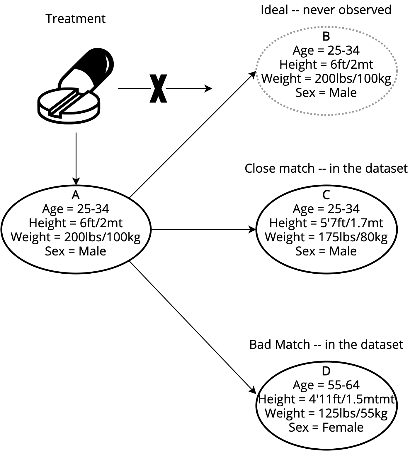 |
Matching: The problem of finding everyone's most similar untreated unit in the dataset
Matching in a nutshell
Matching allows us to take advantage of CI and SUTVA to estimate the CATE in an interpretable way.
- For each unit, $i$ find several other units that are similar in the covariate values.
- Form a Matched Group (MG) with all the units matched to $i$
- Estimate the CATE for $i$ with $$\widehat{CATE}_i = \frac{1}{N^t_{MG}}\sum_{i \in MG}Y_iT_i - \frac{1}{N^c_{MG}}\sum_{i \in MG}Y_i(1-T_i)$$
Why matching?
We choose matching to estimate CATEs because matching is interpretable and interpretability is important
- Interpretability permits greater accountability of decision-makers in high-stake settings
- Interpretability allows researchers to debug their models, datasets and results
- Interpretability makes results from Machine Learning tools more trustworthy to human observers
Matching is interpretable because estimates are case-based
"We came up with that estimates because we looked at these similar cases."
Matching with Continuous Covariates
Problem: do we find know who to match to whom when covariates are continuous?
Solution: Coarsening (binning) variables and then forming matched groups based on bins seems natural
More problems: ...but how do we know how much to coarsen each variable?
Carefully Coarsening Covariates
Consider the problem of having to bin a covariate, $x$
| Fixed boxes | Adaptive boxes |
 |
 |
Takeaways
- Relationship between $x$ and $y$ should be considered when binning
- Even so, optimal-but-fixed width bins are not enough, because...
- Different parts of the covariate space should be binned according to variance of $y$
Takeaways
- Relationship between $x$ and $y$ should be considered when binning
- Even so, optimal-but-fixed width bins are not enough, because...
- Different parts of the covariate space should be binned according to variance of $y$
Adaptive HyperBoxes
[Morucci, Orlandi, Roy, Rudin, Volfovsky (UAI 2020)]
An algorithm to adaptively learn optimal coarsenings of the data that satisfy these criteria.
The AHB Algorithm
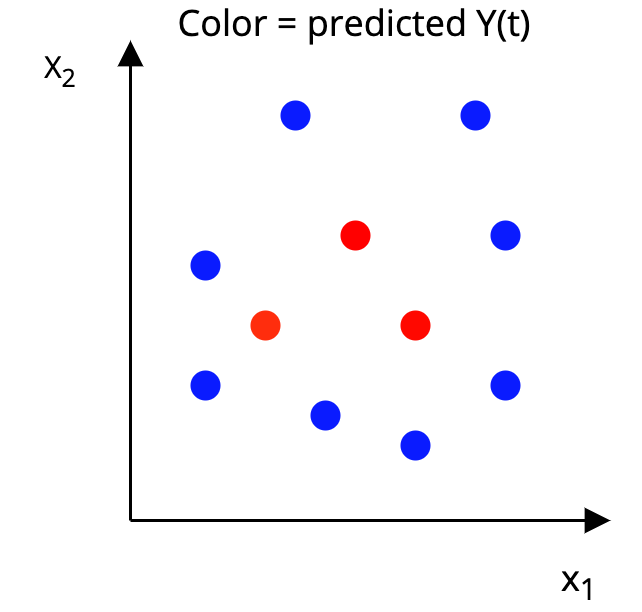
Step 1: On a separate training set, fit a flexible ML model to predict both potential outcomes for each unit in the matching set.

The AHB Algorithm
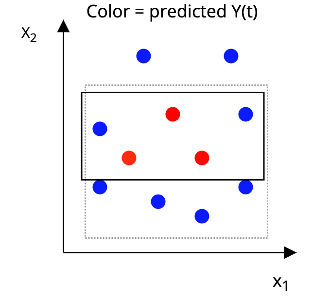
Step 2: Construct a p-dimensional box around each unit, such that, in the box:
|
 |
The AHB Algorithm
Step 2: Construct a p-dimensional box around each unit, such that, in the box:
|
 |
The AHB Algorithm
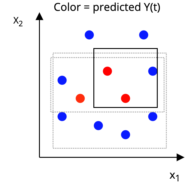
Step 2: Construct a p-dimensional box around each unit, such that, in the box:
|
 |
The AHB Algorithm
Step 2: Construct a p-dimensional box around each unit, such that, in the box:
|
 |
The AHB Algorithm
Step 3: Match together units that are in the same box
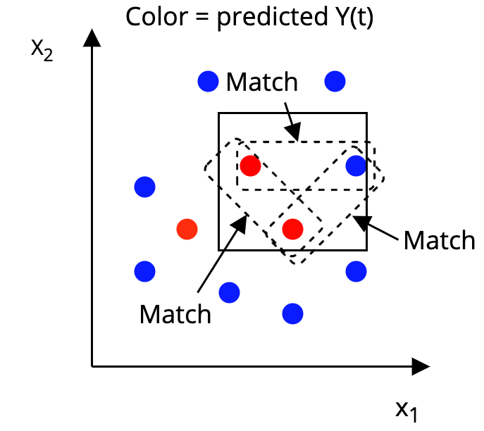
That's it!
AHB Formally
\[\min_{\mathbf{H}} Err(\mathbf{H}, \mathbf{y}) + Var(\mathbf{H}, \mathbf{y}) - n(\mathbf{H})\]
where:
- $\mathbf{H}$ is the hyper-box we want to find
- $Err(\mathbf{H}, \mathbf{y})$ is the outcome prediction error for all points in $\mathbf{H}$
- $Var(\mathbf{H}, \mathbf{y})$ is the outcome variance between points in $\mathbf{H}$
- $n(\mathbf{H})$ is the number of points in $\mathbf{H}$
AHB Formally
In practice, we solve, for every unit, $i$:
\[\min_{\mathbf{H}_i} \sum_{j=1}^n \sum_{t=0}^1 w_{ij}|\hat{f}(\mathbf{x}_i, t) - \hat{f}(\mathbf{x}_j, t)| - \gamma\sum_{j=1}^n w_{ij}\]
- $w_ij$ denotes whether unit $j$ is contained in box $i$
- $\hat{f}(\mathbf{x}, t)$ is the predicted outcome
This function controls all terms previously introduced.
Two solution methods for AHB
An exact solution via a MILP formulation
- Can be solved by any popular MIP solver (CPLEX, Gurobi, GLPK...)
- Simple preprocessing steps make solution relatively fast
Two solution methods for AHB
A fast approximate algorithm
- Determine which unit is closest in absolute distance along each covariate
- Expand the box in the direction with the lowest predicted outcome variance
- Repeat until a desired threshold of matches or loss is met
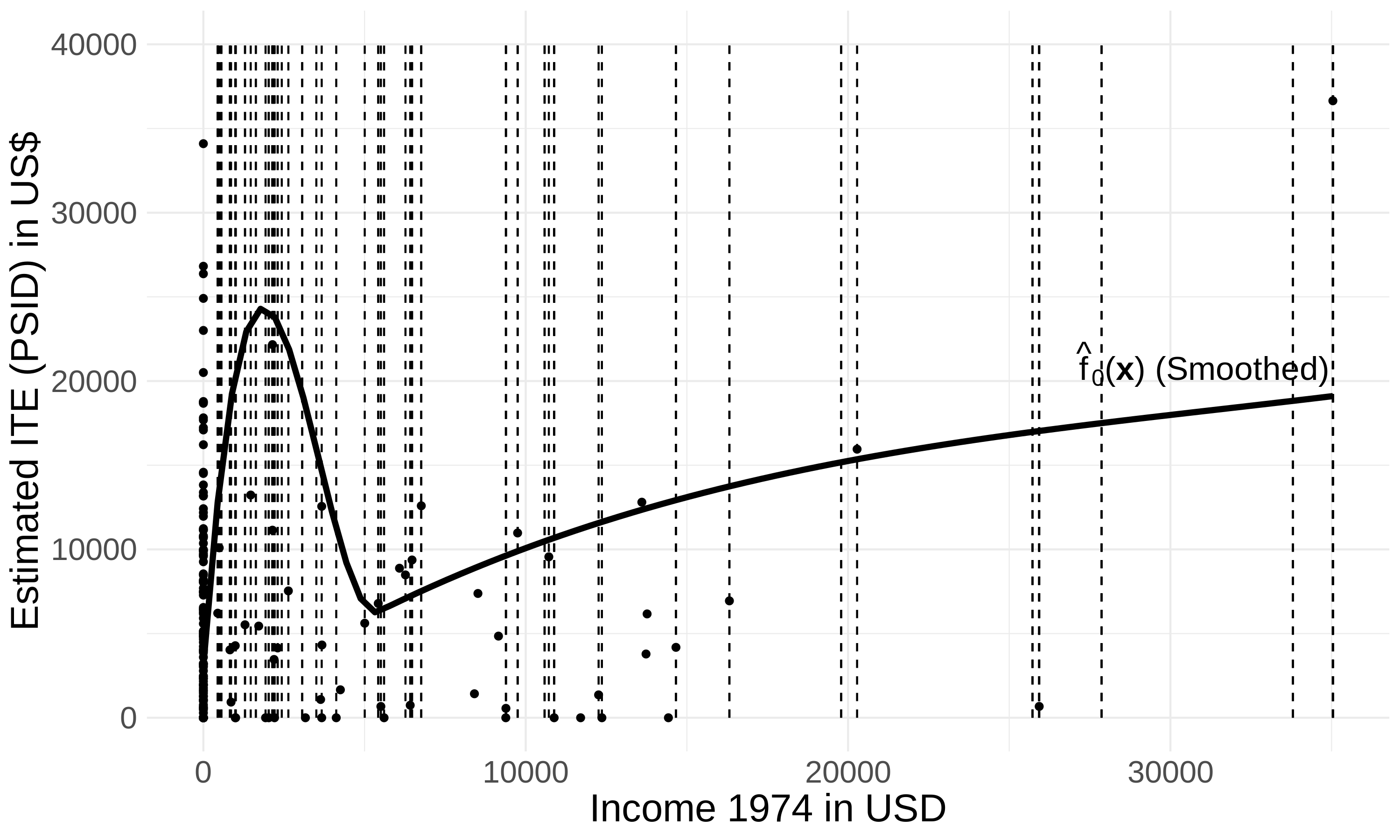
AHB Performance
Test case: Lalonde data
- Effect of training program on income
- Several samples, two observational (PSID, CPS), one experimental (NSW)
- Idea: match experimental treated units (N=185) to observational controls (N>2000) to recover experimental estimates.
- Matching covariates: Age, Education, Prior income, Race, Marital status
AHB Performance
Test case: Lalonde data
Who gets closest to experimental?
| Method | CPS sample | PSID sample |
|---|---|---|
| Experimental | 1794$ | 1794$ |
| AHB | 1720$ | 1762$ |
| Naive | -7729 | -14797 |
| Full Matching | 708 | 816 |
| Prognostic | 1319 | 2224 |
| CEM | 3744 | -2293 |
| Mahalanobis | 1181 | -804 |
AHB Performance
| Recall: ideally, adaptive bins would look like this: | |
| AHB outputs these bins on the Lalonde data: |
 |
Pretty close to the theoretical ideal!
Are our Matches interpretable?
AME/AHB matches vs. Pscore matches
| Age | Education | Black | Married | HS Degree | Pre income | Post Income (outcome) |
| Treated unit we want to match | ||||||
| 22 | 9 | no | no | no | 0 | 3595.89 |
| Matched controls: prognostic score | ||||||
| 44 | 9 | yes | no | no | 0 | 9722 |
| 22 | 12 | yes | no | yes | 532 | 1333.44 |
| 18 | 10 | no | no | no | 0 | 1859.16 |
| Matched controls: AHB | ||||||
| 22 | 9 | no | no | no | 0 | 1245 |
| 20 | 8 | no | no | no | 0 | 5862.22 |
| 24 | 10 | yes | no | no | 0 | 4123.85 |
Are our Matches interpretable?
AHB Interactive output
Software
https://almost-matching-exactly.github.io/Conclusion
Interpretability of causal estimates is important!
- We propose matching methods that produce interpretable and accurate CATE estimates
- Our methods take advantage of machine learning backends to boost accuracy
- Our methods explain both estimates in terms of cases, and why cases were selected in terms of covariate similarity.